The release of .NET Core version 3 contains some exciting cross-platform profiling tools. Today I’ll use some of the newly available tools to target problem areas and improve performance of my F#-based library: FastDtw, as seen here.
The new tooling that supports .NET Core profiling on Linux is a welcome addition. It fills an important gap as the .NET ecosystem further improves support for non-Windows environments. To easily be able to run the entire profilng stack on Linux is a joy. This does require at least .NET Core version 3.0.
To get started I need to add some global tooling. I’ll add the trace tool for data capture and SpeedScope for data viewing. SpeedScope has a website where you can upload traces if you prefer, but I generally like to run things locally if I can.
1 | dotnet tool install --global dotnet-trace--version 3.0.47001 |
Fwiw, Microsoft has released several new tools. Even though I will only focus on trace today, I want to mention the other ones, in case you want to look deeper into them. Counters are for tracking live stats, and Dump is useful for application dumps and debugging.
1 | dotnet tool install --global dotnet-counters --version 3.0.47001 |
Now that the basic tooling is installed, it is time to get started. For this, I’ll put together a simple app that uses the library to profile. Since I want to improve performance along the way, I’ll directly use the project source instead of the nuget package.
1 | dotnet new console -lang f# -n perf && cd perf |
1 | <ItemGroup> |
For my purposes I don’t need anything fancy. I will just loop infinitely, creating 2 randomly sized series to compare. This will give me a steady process to perform a trace against. I could’ve chosen anything really, but opt’d to compare a sin wave to a randomly altered sin wave.
1 | open System |
I’ll open 2 terminals: One to run my test, and another to profile. First, dotnet run to get my simple app looping indefinitely. Tracing is a multi-step process. To start, I need to find it’s process id. Once I have that I can starting tracing the process in question. I also want to save it in a format that speedscope recognizes. Once I have enough data I’ll stop the capture and do some analysis. How much data is enough? That will be problem dependent, but for this particular problem I’ll use about 20 seconds of data. Once the capture is complete, the interesting part starts, looking at the provided profile using speedscope. Running the below command will open the results in a browser.
1 | $ dotnet trace list-processes |
As mentioned before, I am using speedscope, which is a flamegraph visualizer. I have the data in the proper format, but if I didn’t, the trace tool comes with a conversion command as well, dotnet trace convert trace.foo --format speedscope.
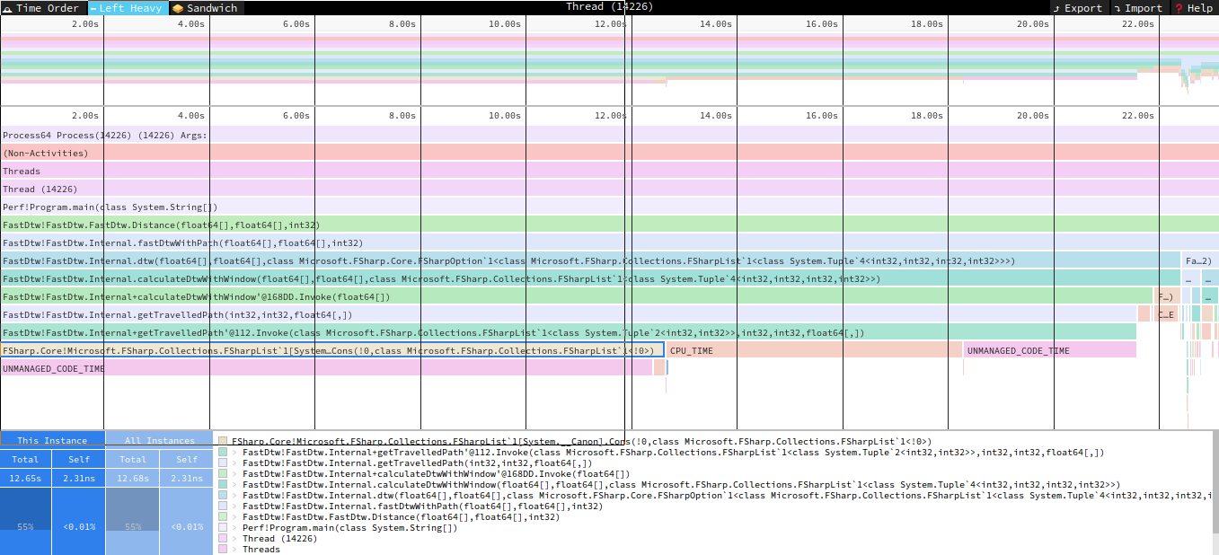
My intention is not to make a speedscope tutorial, but it is useful to get some bearings. The interface has 3 main views “Time Order”, “Left Heavy”, and “Sandwich”. Time Order is representative of chronological time through the execution of the application, which isn’t interesting to me today. Left Heavy groups function calls so it is easy to see which functions are taking the most time, and their respective callers. “Sandwich” uses a percent time execution to find the big timesinks, but it also includes callers and callees, to help track the call stack a bit. Depending on the view that is picked, additional detail is shown regarding the function in question. I will primary leverage the last two views.
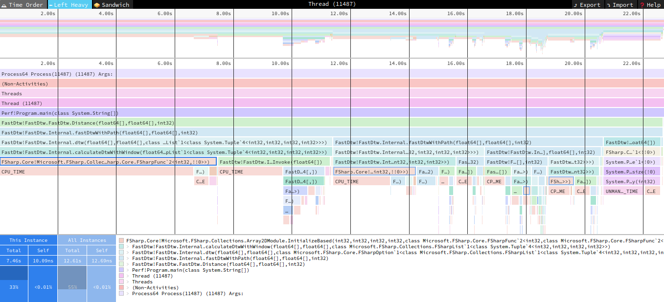
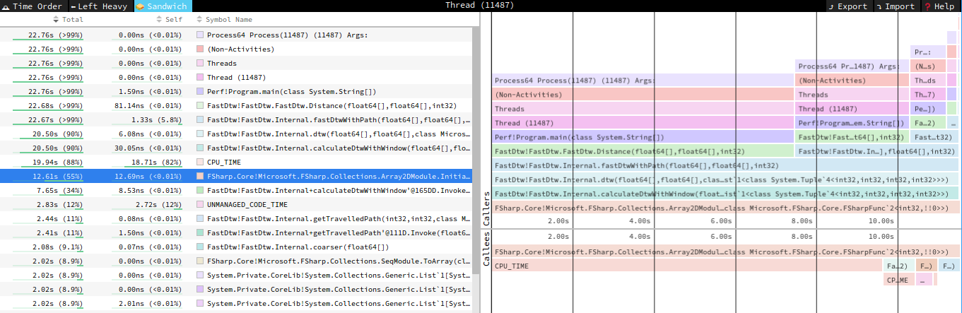
Looking at the above charts, it appears Array2D creation is unexpectedly taking a significant amount of time. Looking into the code I see a frankly silly mistake. I want to initialize the array with 0s, but for some reason I was using a lambda function instead of a straight initialization. I don’t need the additional functionality of the lambda so this is a pretty obvious change. As a sidenote, the create runs about 60% faster than init in my very informal tests.
1 | // OLD |
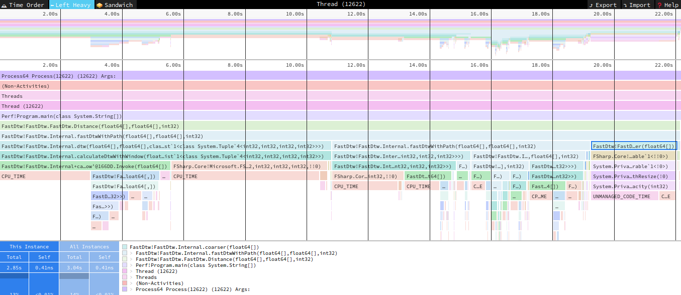
I now rerun my test with the newly enhanced code to find another area of contention in the coarser function. Here is another interesting find, apparently a stepped population of an array triggers an underlying list creation, which carries with it some additional overhead. Initializing the array differently is about 10 times faster than the [| a .. s .. b |]. I think the original code is a bit more intuitive, but the change is worth the performance boost.
1 | // OLD |
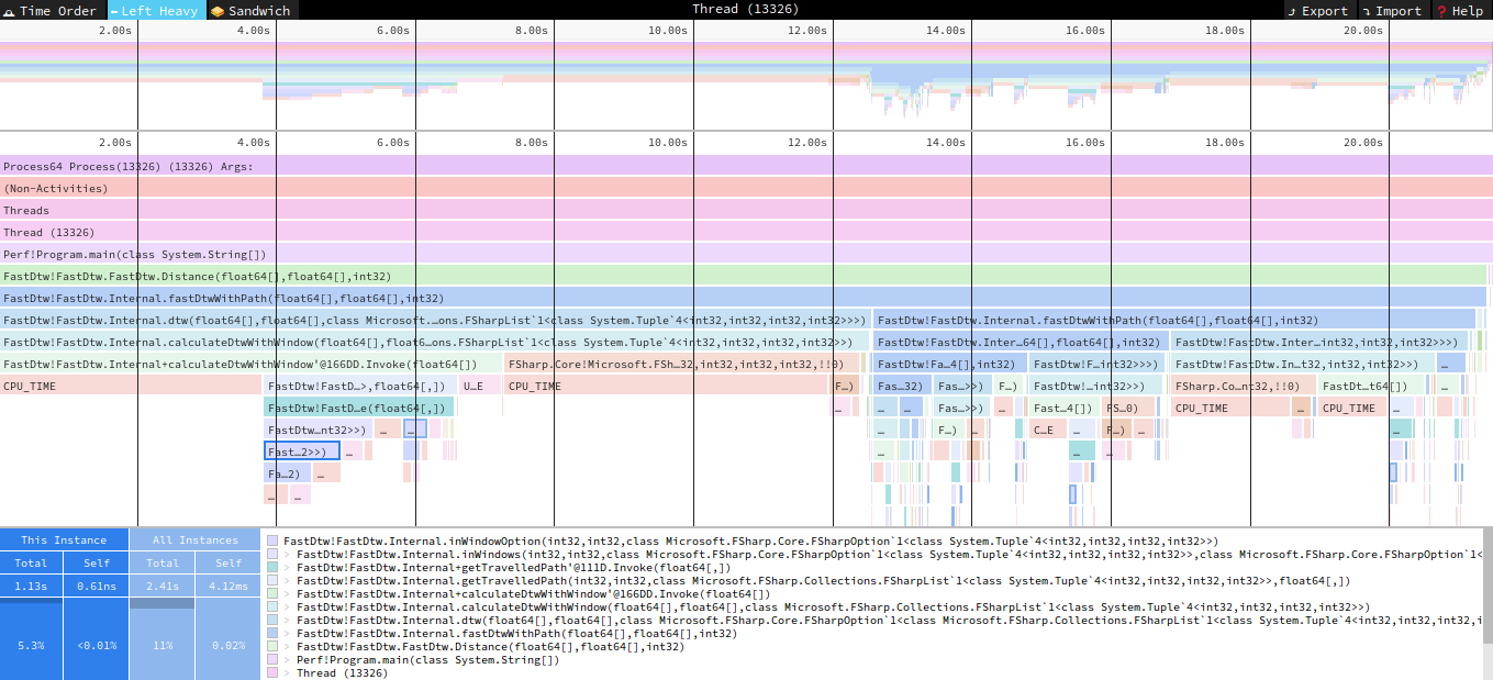
In the next profiling run, I see calls being dominated by my InWindow functions. Internally they mostly use match against an option type. Turns out using a straight If x.IsSome then ... else ... is about 3 times faster than the equivalent match. I will admit, I have a tendancy to over-use match, this is a good reminder to be more careful and ensure the usecase makes sense. This brings up another rework, the travelledPath function I have for backtracking the path used by the algorithm for determining distance between the series. In retrospect I overthought things. I won’t show the before/after code because it’s a larger rewrite. I was able to simplify and make the function faster, ironically removing a several match option calls that initially pointed me this way.
1 | // Old |
This is where I come to an end for now. I allocated myself a limited amount of weekend time for this. It looks like the next big enhancement is to remove a list usage, but the implications of that change are larger than I’m willing to take on in my current timeframe. I will mark this away as a future enhancement. I’m pretty happy with what I found, with not that much effort. The new dotnet trace tool, in combination with speedscope, has proven to be very useful in quick profiling iterations on Linux. Now that the optimizations are complete, it would be nice to see a before/after comparison. For this I’ll use BenchmarkDotNet for some comparative analysis. After putting together a quick benchmark app, here are the results. Running on a couple different series sizes, I see about a 25% to 30% performance boost.
1 | | Method | SeriesSize | Mean | Error | StdDev | Gen 0 | Gen 1 | Gen 2 | Allocated | |
This is all the performance tuning I have for today. My goal was to find some easy wins, and I did that. It has been a nice little project to kick the new performance tooling tires. I hope you’ve also found this interesting and I encourage you to check them out. I think you’ll find they are a nice addition to the toolkit.